Striatum subregion analysis

Break down projection density by anatomical subdivisions of the caudate putamen (CP) and nucleus accumbens (NAc) using the Allen v2 atlas, with optional CSV export.

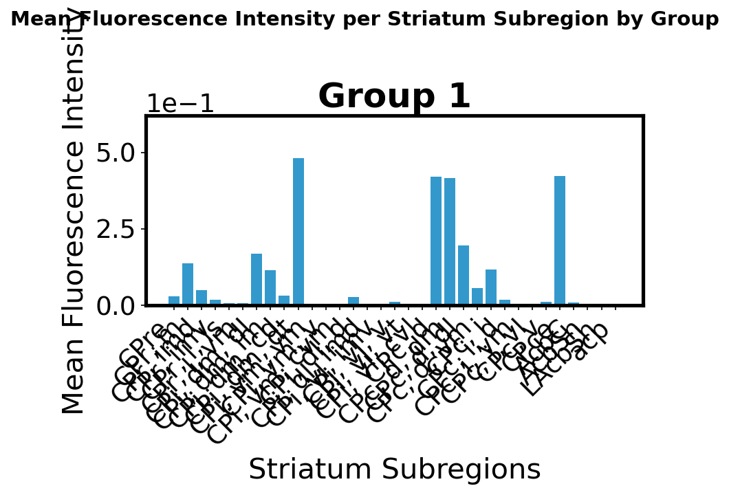
Mean fluorescence intensity per striatum subregion for projections from all visual cortical areas to CP and NAc. Subregions are defined by the Allen v2 atlas.

Requires the Allen v2 atlas files (annotation_volume_v2_20um_by_index.npy and UnifiedAtlas_Label_ontology_v2.csv) placed in a separate directory (allen_atlas_path_v2). These files must be downloaded manually — they are not auto-downloaded.

Python:

# First get the projection matrix from plot_connectivity
(proj_matrix,   # ndarray (n_slices x n_bins x n_bins x groups): binned projection density per slice
 proj_coords    # list of bin edge arrays: spatial coordinates of each slice panel
) = bsv.plot_connectivity(
    experiment_data=experiment_imgs,
    allen_atlas_path='/path/to/allenCCF',    # atlas files auto-downloaded here on first use
    output_region='CP',
    number_of_chunks=10,                     # number of evenly spaced slices to display
    number_of_pixels=15,                     # number of 2D histogram bins per axis per slice (bin size adapts to region extent)
    plane='coronal',
    region_only=True,
    smoothing=2,
    color_limits='global',
    color=None,
    normalization_info='injectionIntensity')

# Analyze subregions
(subregion_results,  # dict: mean fluorescence per CP/NAc subregion per group
 global_results      # dict: whole-region summary statistics
) = bsv.analyze_cp_subregions(
    projection_matrix_array=proj_matrix,
    projection_matrix_coordinates_ara=proj_coords,
    allen_atlas_path_v2='/path/to/allenCCF_v2')  # v2 atlas dir — must be downloaded manually

# Export to CSV
subregion_results, global_results = bsv.analyze_cp_subregions(
    projection_matrix_array=proj_matrix,
    projection_matrix_coordinates_ara=proj_coords,
    allen_atlas_path_v2='/path/to/allenCCF_v2',
    save_csv_path='/path/to/output.csv')

# Or do plot + analysis in one step
proj_matrix, proj_coords, sub_results, glob_results = \
    bsv.plot_connectivity_with_subregion_analysis(
        experiment_data=experiment_imgs,
        allen_atlas_path='/path/to/allenCCF',
        allen_atlas_path_v2='/path/to/allenCCF_v2',
        output_region='CP',
        number_of_chunks=10,
        number_of_pixels=15,
        plane='coronal',
        region_only=True,
        smoothing=2,
        color_limits='global',
        color=None,
        normalization_info='injectionIntensity')

The exported CSV contains one row per striatum subregion with its GlobalMeanIntensity (mean projection fluorescence across all analysed voxels of that subregion) and TotalVoxelCount, sorted from strongest to weakest. A companion *_nonzero.csv is also written containing only subregions that received signal. The returned global_results dict holds the same per-subregion summary intensities, while subregion_results breaks them down per group (e.g. per injection-AP group) and per slice.

MATLAB:

[projMatrix, projCoords] = bsv.plotConnectivity(experimentImgs, allenAtlasPath, ...
    'CP', 10, 15, 'coronal', true, 2, 'global', [], 'injectionIntensity');

[subResults, globalResults] = bsv.analyzeCPSubregions(projMatrix, projCoords, ...
    allenAtlasPath_v2, [], inputRegions, [], csvPath);